When talking about used configurations we refer to all the arrays of electrodes used to obtain the apparent resistivity, which are basically superposition of the fundamental equation for the potential from a current source with appropriate sign for the current.
The formulas for apparent resistivity are a product of the impedance V/I (Ohms) and a geometric factor with the units of length (meters). To investigate the resistivity distribution with depth, called a sounding, the arrays are expanded about a center point and the apparent resistivities are plotted vs. spacing usually on a log-log plot.
As a general rule, the apparent resistivities are plotted as a function of array spacing and lateral position using plotting conventions that have become accepted for each type of array.
Pole – Pole
The simplest array is one in which one of the current electrodes and one of the potential electrodes are placed so far away that they can be considered at infinity. This configuration with its formula for apparent resistivity is shown below.
Roa = V/I*2PIa

This array can actually be achieved for surveys of small overall dimension when it is possible to put the distant electrodes some practical distance away. For a survey in an area of a few square meters infinity can be on the order of a hundred meters. Pole-pole sounding data is plotted as apparent resistivity vs. “a”.
Pole – Dipole
If only one of the current electrodes is placed at infinity the configuration and the apparent resistivity are as shown:
Roa = 2*PI*[b(a+b)/a]*V/I
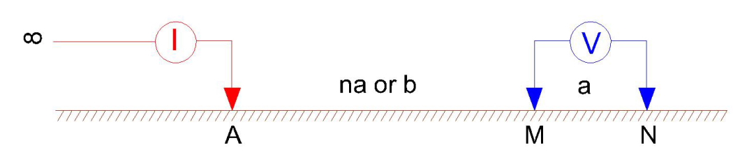
This array is used frequently in resistivity surveying and the spacing are usually described, and taken, in integer multiples of the voltage electrode spacing b = na. The standard nomenclature is to call the potential electrode spacing “a” so the configuration and apparent resistivity becomes:
Roa = 2*PI*an(n+1)*V/I
Pole-dipole sounding data is plotted as apparent resistivity vs. “a”.
Wenner
It is now seen to be a simple variant of the pole-dipole in which the distant pole at infinity is brought in and all the electrodes are given the same spacing, “a”, as seen in the following configuration:
Roa = 2*PI*a*V/I

The Wenner array is normally used for sounding and the apparent resistivities are plotted vs. “a” such as is shown in figure.
Schlumberger
One of the first arrays used in the 1920 and still popular today is the Schlumberger array shown below with its formula for apparent resistivity. It is another variant of the pole-dipole, again with the second current electrode placed symmetrically opposite the first. The voltage difference is consequently doubled and so the apparent resistivity is the same as that for the general pole-dipole with a factor of 1/2 in the geometric factor. In a Schlumberger sounding the voltage electrodes are usually kept small and fixed while only the “b” spacing is changed.
Roa = V/I*PI*b(b+a)/a

Further, it is conventional to consider the spacing “b” to be the distance from the center of the array to the outermost electrodes. In this case “b” in the above expressions becomes AB/2. If a << AB/2 the above formulas for Roa are changed:
Roa = V/I*PI* b^2/a if a<<b
Data from a Schlumberger sounding is plotted vs. spacing in the same manner as the Wenner data of figure.
Dipole – Dipole
The dipole – dipole array is logistically the most convenient in the field, especially for large spacing. All the other arrays require significant lengths of wire to connect the power supply and voltmeter to their respective electrodes and these wires must be moved for every change in spacing as the array is either expanded for a sounding or moved along a line. The convention for the dipole-dipole array shown below is that current and voltage spacing is the same, “a”, and the spacing between them is an integer multiple of “a”.
The apparent resistivity is given by:
Roa = V/I*PI*an(n+1)(n+2)

Hummel
It is actually a more practical variant of the Schlumberger array, easy to adapt to difficult working conditions. In practical terms is a half of the Schlumberger array, one of the power electrodes being placed at infinity perpendicular on direction of the array.
The computing of the apparent resistivity is done using the same formula as for the Schlumberger array, but to be accurate the resistivity is doubled.
Roa = 2* V/I*PI* b^2/a
Using this method we can reduce the personal number necessary for the operation of moving the electrodes and also the measuring time. This technique is useful when the geological conditions allow its use – relative horizontal layers.